what is the probability that the random variable will assume a value between and (to 4 decimals)

five.3 Probability Computations for General Normal Random Variables

Learning Objective

1. To learn how to compute probabilities related to whatever normal random variable.

If X is whatever usually distributed normal random variable then Effigy 12.ii "Cumulative Normal Probability" can too be used to compute a probability of the form $P\left(a<X<b\right)$ past means of the following equality.

If X is a unremarkably distributed random variable with mean μ and standard difference σ, and then

$$P\left(a<X<b\right)=P(\frac{a-\mathit{\mu }}{\mathit{\sigma }}<Z<\frac{b-\mathit{\mu }}{\mathit{\sigma }})$$

where Z denotes a standard normal random variable. a can be any decimal number or $\text{−}\infty$ ; b can be any decimal number or $\infty .$

The new endpoints $\left(a-\mathit{\mu }\right)∕\mathit{\sigma }$ and $\left(b-\mathit{\mu }\right)∕\mathit{\sigma }$ are the z-scores of a and b as divers in Section two.4.2 in Chapter 2 "Descriptive Statistics".

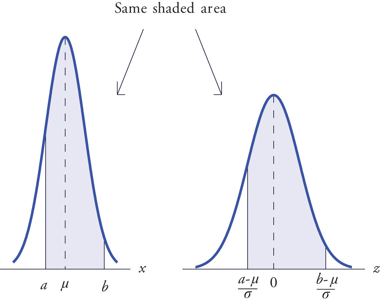
Effigy 5.14 "Probability for an Interval of Finite Length" illustrates the pregnant of the equality geometrically: the ii shaded regions, 1 under the density curve for X and the other nether the density curve for Z, have the aforementioned area. Instead of drawing both bell curves, though, we will always draw a single generic bell-shaped bend with both an x-axis and a z-axis below it.

Figure 5.14 Probability for an Interval of Finite Length

Example 9

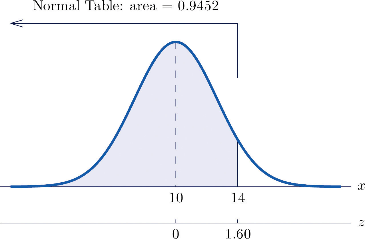
Let X be a normal random variable with mean μ = 10 and standard divergence σ = 2.five. Compute the post-obit probabilities.

1. P(10 < 14).
2. $P\left(\mathrm{eight}<X<14\right).$

Solution:

1. Come across Figure five.fifteen "Probability Computation for a General Normal Random Variable".

   $$\begin{array}{lll}\hfill P\left(\mathrm{10}<14\right)& =& P\left(\right.Z<\frac{14-\mathit{\mu }}{\mathit{\sigma }}\left)\right.\\ & =& P\left(\right.Z<\frac{14-10}{\mathrm{2.v}}\left)\right.\\ & =& P\left(Z<\mathrm{1.lx}\right)\\ & =& 0.9452\end{array}$$

Figure 5.fifteen Probability Ciphering for a Full general Normal Random Variable

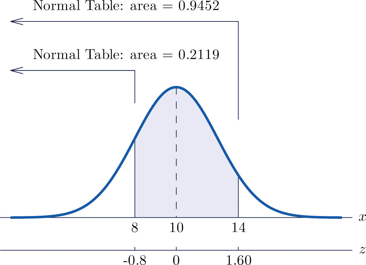
1. Come across Figure 5.16 "Probability Ciphering for a Full general Normal Random Variable".

   $$\begin{array}{lll}\hfill P\left(\mathrm{viii}<X<\mathrm{fourteen}\right)& =& P\left(\right.\frac{\mathrm{eight}-10}{\mathrm{ii.5}}<Z<\frac{14-10}{\mathrm{2.five}}\left)\right.\\ & =& P\left(\text{−}\mathrm{0.lxxx}<Z<\mathrm{1.lx}\right)\\ & =& 0.9452-0.2119\\ & =& 0.7333\end{array}$$

Figure 5.16 Probability Ciphering for a General Normal Random Variable

Example 10

The lifetimes of the tread of a certain automobile tire are normally distributed with mean 37,500 miles and standard deviation 4,500 miles. Find the probability that the tread life of a randomly selected tire will be betwixt xxx,000 and 40,000 miles.

Solution:

Permit X announce the tread life of a randomly selected tire. To brand the numbers easier to work with we volition choose thousands of miles as the units. Thus μ = 37.5, σ = four.5, and the problem is to compute $P\left(\mathrm{xxx}<\mathrm{10}<40\right).$ Figure 5.17 "Probability Computation for Tire Tread Wear" illustrates the following computation:

Figure 5.17 Probability Computation for Tire Tread Wear

$$\begin{array}{lll}\hfill P\left(\mathrm{thirty}<X<40\right)& =& P\left(\right.\frac{\mathrm{thirty}-\mathit{\mu }}{\mathit{\sigma }}<Z<\frac{\mathrm{xl}-\mathit{\mu }}{\mathit{\sigma }}\left)\right.\\ & =& P\left(\right.\frac{30-37.5}{\mathrm{4.five}}<Z<\frac{\mathrm{xl}-\mathrm{37.five}}{\mathrm{4.five}}\left)\right.\\ & =& P\left(\text{−}1.67<Z<0.56\right)\\ & =& 0.7123-0.0475\\ & =& 0.6648\end{array}$$

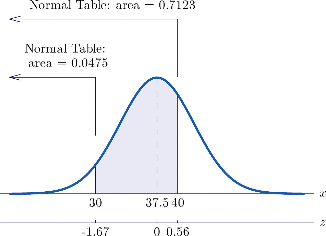
Note that the two z-scores were rounded to 2 decimal places in order to utilize Effigy 12.2 "Cumulative Normal Probability".

Case eleven

Scores on a standardized college archway test (CEE) are normally distributed with mean 510 and standard divergence 60. A selective academy considers for admission only applicants with CEE scores over 650. Find percentage of all individuals who took the CEE who meet the university'due south CEE requirement for consideration for access.

Solution:

Allow X announce the score made on the CEE by a randomly selected private. And so 10 is normally distributed with mean 510 and standard divergence 60. The probability that Ten prevarication in a detail interval is the same as the proportion of all exam scores that lie in that interval. Thus the solution to the problem is P(X > 650), expressed as a percentage. Figure 5.18 "Probability Computation for Exam Scores" illustrates the following computation:

Figure 5.18 Probability Ciphering for Exam Scores

$$\begin{array}{lll}\hfill P\left(X>650\right)& =& P\left(\right.Z>\frac{650-\mathit{\mu }}{\mathit{\sigma }}\left)\right.\\ & =& P\left(\right.Z>\frac{650-510}{60}\left)\right.\\ & =& P\left(Z>2.33\right)\\ & =& \mathrm{one}-0.9901\\ & =& 0.0099\end{array}$$

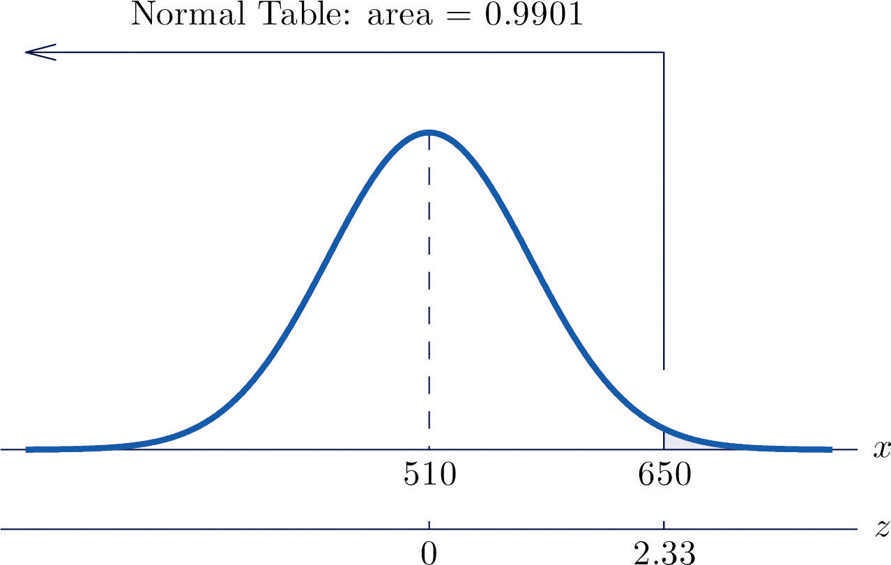
The proportion of all CEE scores that exceed 650 is 0.0099, hence 0.99% or about 1% practise.

Exercises

Basic

1. 10 is a normally distributed random variable with hateful 57 and standard deviation 6. Find the probability indicated.

   1. P(Ten < 59.5)
   2. P(X < 46.2)
   3. P(X > 52.2)
   4. P(X > seventy)

2. X is a normally distributed random variable with hateful −25 and standard divergence 4. Notice the probability indicated.

   1. P(X < −27.ii)
   2. P(X < −fourteen.viii)
   3. P(Ten > −33.ane)
   4. P(X > −sixteen.v)

3. X is a normally distributed random variable with hateful 112 and standard deviation 15. Observe the probability indicated.

   1. $P\left(100<X<125\right)$
   2. $P\left(91<\mathrm{10}<107\right)$
   3. $P\left(118<X<160\right)$

4. X is a normally distributed random variable with mean 72 and standard deviation 22. Find the probability indicated.

   1. $P\left(78<X<127\right)$
   2. $P\left(60<X<90\right)$
   3. $P\left(49<X<71\right)$

5. Ten is a normally distributed random variable with mean 500 and standard deviation 25. Find the probability indicated.

   1. P(X < 400)
   2. $P\left(466<X<625\right)$

6. X is a normally distributed random variable with mean 0 and standard deviation 0.75. Notice the probability indicated.

   1. P(−iv.02 < Ten < 3.82)
   2. P(X > 4.11)

7. X is a unremarkably distributed random variable with mean xv and standard departure 1. Use Figure 12.ii "Cumulative Normal Probability" to observe the first probability listed. Find the second probability using the symmetry of the density curve. Sketch the density curve with relevant regions shaded to illustrate the computation.

   1. P(X < 12), P(10 > 18)
   2. P(Ten < xiv), P(Ten > 16)
   3. P(Ten < 11.25), P(Ten > 18.75)
   4. P(X < 12.67), P(10 > 17.33)

8. X is a commonly distributed random variable with mean 100 and standard deviation 10. Use Figure 12.2 "Cumulative Normal Probability" to find the first probability listed. Find the 2d probability using the symmetry of the density curve. Sketch the density curve with relevant regions shaded to illustrate the computation.

   1. P(X < 80), P(X > 120)
   2. P(Ten < 75), P(10 > 125)
   3. P(X < 84.55), P(10 > 115.45)
   4. P(Ten < 77.42), P(10 > 122.58)

9. X is a normally distributed random variable with mean 67 and standard departure thirteen. The probability that X takes a value in the union of intervals $\left(\text{−}\infty ,67-a\right]\cup \left[67+a,\infty \right)$ will be denoted $P\left(\mathrm{Ten}\le 67-a\text{or}X\ge 67+a\right).$ Use Effigy 12.2 "Cumulative Normal Probability" to detect the following probabilities of this type. Sketch the density curve with relevant regions shaded to illustrate the computation. Because of the symmetry of the density curve yous need to employ Figure 12.two "Cumulative Normal Probability" just in one case for each part.

   1. $P\left(X<57\text{or}X>77\right)$
   2. $P\left(\mathrm{10}<47\text{or}\mathrm{10}>87\right)$
   3. $P\left(X<49\text{or}X>85\right)$
   4. $P\left(X<37\text{or}X>97\right)$

10. X is a ordinarily distributed random variable with hateful 288 and standard deviation 6. The probability that X takes a value in the matrimony of intervals $\left(\text{−}\infty ,288-a\right]\cup \left[288+a,\infty \right)$ will be denoted $P\left(\mathrm{Ten}\le 288-a\text{or}X\ge 288+a\right).$ Use Figure 12.2 "Cumulative Normal Probability" to discover the post-obit probabilities of this blazon. Sketch the density curve with relevant regions shaded to illustrate the computation. Because of the symmetry of the density curve y'all need to use Figure 12.2 "Cumulative Normal Probability" only in one case for each part.

    1. $P\left(X<278\text{or}X>298\right)$
    2. $P\left(X<268\text{or}X>308\right)$
    3. $P\left(X<273\text{or}X>303\right)$
    4. $P\left(\mathrm{10}<280\text{or}X>296\right)$

Applications

11. The amount X of beverage in a can labeled 12 ounces is usually distributed with mean 12.i ounces and standard deviation 0.05 ounce. A can is selected at random.

    1. Find the probability that the can contains at least 12 ounces.
    2. Notice the probability that the can contains between eleven.9 and 12.1 ounces.

12. The length of gestation for swine is ordinarily distributed with mean 114 days and standard deviation 0.75 twenty-four hours. Find the probability that a litter will exist built-in within one 24-hour interval of the mean of 114.

13. The systolic blood pressure 10 of adults in a region is normally distributed with mean 112 mm Hg and standard deviation 15 mm Hg. A person is considered "prehypertensive" if his systolic blood pressure is between 120 and 130 mm Hg. Find the probability that the blood force per unit area of a randomly selected person is prehypertensive.

14. Heights 10 of adult women are normally distributed with mean 63.7 inches and standard departure two.71 inches. Romeo, who is 69.25 inches tall, wishes to date only women who are shorter than he but inside 4 inches of his top. Discover the probability that the next woman he meets will have such a top.

15. Heights X of adult men are commonly distributed with hateful 69.1 inches and standard deviation 2.92 inches. Juliet, who is 63.25 inches tall, wishes to engagement just men who are taller than she merely within 6 inches of her height. Notice the probability that the next man she meets will take such a height.

16. A regulation hockey puck must weigh between five.5 and half dozen ounces. The weights 10 of pucks fabricated by a particular process are unremarkably distributed with hateful 5.75 ounces and standard divergence 0.xi ounce. Observe the probability that a puck made by this process volition run across the weight standard.

17. A regulation golf ball may not weigh more than 1.620 ounces. The weights Ten of golf balls made by a item process are usually distributed with mean 1.361 ounces and standard divergence 0.09 ounce. Find the probability that a golf game ball fabricated by this process will encounter the weight standard.

18. The length of fourth dimension that the battery in Hippolyta'south cell telephone will hold enough charge to operate acceptably is ordinarily distributed with mean 25.half dozen hours and standard deviation 0.32 hour. Hippolyta forgot to charge her phone yesterday, so that at the moment she offset wishes to use it today it has been 26 hours 18 minutes since the phone was last fully charged. Discover the probability that the telephone will operate properly.

19. The amount of non-mortgage debt per household for households in a detail income subclass in 1 office of the land is ordinarily distributed with mean $28,350 and standard departure $three,425. Find the probability that a randomly selected such household has between $xx,000 and $30,000 in not-mortgage debt.

20. Birth weights of full-term babies in a certain region are normally distributed with mean 7.125 lb and standard deviation 1.290 lb. Find the probability that a randomly selected newborn will weigh less than 5.five lb, the celebrated definition of prematurity.

21. The altitude from the seat back to the forepart of the knees of seated adult males is normally distributed with mean 23.8 inches and standard deviation 1.22 inches. The altitude from the seat back to the back of the side by side seat forward in all seats on aircraft flown by a upkeep airline is 26 inches. Find the proportion of adult men flight with this airline whose knees volition touch the dorsum of the seat in front of them.

22. The altitude from the seat to the acme of the caput of seated developed males is ordinarily distributed with mean 36.five inches and standard difference 1.39 inches. The altitude from the seat to the roof of a particular brand and model auto is xl.5 inches. Discover the proportion of developed men who when sitting in this car will have at least one inch of headroom (distance from the top of the head to the roof).

Additional Exercises

23. The useful life of a particular brand and type of automotive tire is normally distributed with hateful 57,500 miles and standard difference 950 miles.

    1. Find the probability that such a tire will have a useful life of between 57,000 and 58,000 miles.
    2. Hamlet buys four such tires. Assuming that their lifetimes are independent, observe the probability that all four will last betwixt 57,000 and 58,000 miles. (If so, the best tire will accept no more than 1,000 miles left on it when the outset tire fails.) Hint: There is a binomial random variable here, whose value of p comes from part (a).

24. A car produces large fasteners whose length must be within 0.v inch of 22 inches. The lengths are ordinarily distributed with hateful 22.0 inches and standard deviation 0.17 inch.

    1. Find the probability that a randomly selected fastener produced by the machine will take an acceptable length.
    2. The motorcar produces xx fasteners per hour. The length of each one is inspected. Bold lengths of fasteners are independent, find the probability that all 20 will accept acceptable length. Hint: There is a binomial random variable here, whose value of p comes from role (a).

25. The lengths of time taken by students on an algebra proficiency exam (if not forced to terminate before completing it) are ordinarily distributed with mean 28 minutes and standard deviation i.five minutes.

    1. Discover the proportion of students who will terminate the examination if a 30-infinitesimal time limit is set.
    2. Half dozen students are taking the exam today. Notice the probability that all half dozen will finish the exam within the 30-minute limit, assuming that times taken past students are independent. Hint: There is a binomial random variable here, whose value of p comes from part (a).

26. Heights of developed men between 18 and 34 years of age are normally distributed with mean 69.one inches and standard difference two.92 inches. One requirement for enlistment in the military is that men must stand between 60 and fourscore inches tall.

    1. Find the probability that a randomly elected homo meets the height requirement for military service.
    2. Twenty-three men independently contact a recruiter this week. Notice the probability that all of them meet the height requirement. Hint: At that place is a binomial random variable here, whose value of p comes from role (a).

27. A regulation hockey puck must weigh betwixt 5.5 and 6 ounces. In an alternative manufacturing procedure the mean weight of pucks produced is 5.75 ounce. The weights of pucks take a normal distribution whose standard deviation tin can be decreased past increasingly stringent (and expensive) controls on the manufacturing process. Find the maximum allowable standard deviation then that at near 0.005 of all pucks will fail to run into the weight standard. (Hint: The distribution is symmetric and is centered at the middle of the interval of adequate weights.)

28. The amount of gasoline X delivered past a metered pump when it registers 5 gallons is a normally distributed random variable. The standard departure σ of X measures the precision of the pump; the smaller σ is the smaller the variation from delivery to delivery. A typical standard for pumps is that when they show that 5 gallons of fuel has been delivered the actual corporeality must be between iv.97 and 5.03 gallons (which corresponds to being off past at most virtually half a cup). Supposing that the mean of 10 is v, detect the largest that σ can be and then that P(four.97 < Ten < 5.03) is 1.0000 to four decimal places when computed using Figure 12.2 "Cumulative Normal Probability", which means that the pump is sufficiently authentic. (Hint: The z-score of v.03 will be the smallest value of Z so that Figure 12.2 "Cumulative Normal Probability" gives $P\left(Z<z\right)=1.0000.$ )

Answers

1. 1. 0.6628
   2. 0.0359
   3. 0.7881
   4. 0.0150
3. 1. 0.5959
   2. 0.2899
   3. 0.3439
5. 1. 0.0000
   2. 0.9131
7. 1. 0.0013, 0.0013
   2. 0.1587, 0.1587
   3. 0.0001, 0.0001
   4. 0.0099, 0.0099
9. 1. 0.4412
   2. 0.1236
   3. 0.1676
   4. 0.0208

11. 1. 0.9772
    2. 0.5000

13. 0.1830

15. 0.4971

17. 0.9980

19. 0.6771

21. 0.0359

23. 1. 0.4038
    2. 0.0266
25. 1. 0.9082
    2. 0.5612

27. 0.089

biseyoubety.blogspot.com

Source: https://saylordotorg.github.io/text_introductory-statistics/s09-03-probability-computations-for-g.html

Share this post